Month: July 2018

Linear Search Algorithm | Example | Time Complexity

Searching-


  • Searching is a process of finding a particular element among several given elements.
  • The search is successful if the required element is found.
  • Otherwise, the search is unsuccessful.


Searching Algorithms-


Searching Algorithms are a family of algorithms used for the purpose of searching.

The searching of an element in the given array may be carried out in the following two ways-


  1. Linear Search
  2. Binary Search


In this article, we will discuss about Linear Search Algorithm.


Linear Search-


  • Linear Search is the simplest searching algorithm.
  • It traverses the array sequentially to locate the required element.
  • It searches for an element by comparing it with each element of the array one by one.
  • So, it is also called as Sequential Search.


Linear Search Algorithm is applied when-

  • No information is given about the array.
  • The given array is unsorted or the elements are unordered.
  • The list of data items is smaller.


Linear Search Algorithm-


Consider-

  • There is a linear array ‘a’ of size ‘n’.
  • Linear search algorithm is being used to search an element ‘item’ in this linear array.
  • If search ends in success, it sets loc to the index of the element otherwise it sets loc to -1.


Then, Linear Search Algorithm is as follows-


Linear_Search (a , n , item , loc)


Begin

for i = 0 to (n - 1) by 1 do

    if (a[i] = item) then

        set loc = i

        Exit

    endif

endfor

set loc = -1

End


Time Complexity Analysis-


Linear Search time complexity analysis is done below-


Best case-


In the best possible case,

  • The element being searched may be found at the first position.
  • In this case, the search terminates in success with just one comparison.
  • Thus in best case, linear search algorithm takes O(1) operations.


Worst Case-


In the worst possible case,

  • The element being searched may be present at the last position or not present in the array at all.
  • In the former case, the search terminates in success with n comparisons.
  • In the later case, the search terminates in failure with n comparisons.
  • Thus in worst case, linear search algorithm takes O(n) operations.


Thus, we have-


Time Complexity of Linear Search Algorithm is O(n).

Here, n is the number of elements in the linear array.


Linear Search Efficiency-


  • Linear Search is less efficient when compared with other algorithms like Binary Search & Hash tables.
  • The other algorithms allow significantly faster searching.


Linear Search Example-


Consider-

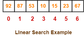
  • We are given the following linear array.
  • Element 15 has to be searched in it using Linear Search Algorithm.


Now,

  • Linear Search algorithm compares element 15 with all the elements of the array one by one.
  • It continues searching until either the element 15 is found or all the elements are searched.


Linear Search Algorithm works in the following steps-


Step-01:


  • It compares element 15 with the 1st element 92.
  • Since 15 ≠ 92, so required element is not found.
  • So, it moves to the next element.


Step-02:


  • It compares element 15 with the 2nd element 87.
  • Since 15 ≠ 87, so required element is not found.
  • So, it moves to the next element.


Step-03:


  • It compares element 15 with the 3rd element 53.
  • Since 15 ≠ 53, so required element is not found.
  • So, it moves to the next element.


Step-04:


  • It compares element 15 with the 4th element 10.
  • Since 15 ≠ 10, so required element is not found.
  • So, it moves to the next element.


Step-05:


  • It compares element 15 with the 5th element 15.
  • Since 15 = 15, so required element is found.
  • Now, it stops the comparison and returns index 4 at which element 15 is present.


To gain better understanding about Linear Search Algorithm,

Watch this Video Lecture


Next Article- Binary Search


Get more notes and other study material of Design and Analysis of Algorithms.

Watch video lectures by visiting our YouTube channel LearnVidFun.
Recursion Tree | Solving Recurrence Relations

Recursion Tree-


  • Like Master’s Theorem, Recursion Tree is another method for solving the recurrence relations.
  • A recursion tree is a tree where each node represents the cost of a certain recursive sub-problem.
  • We sum up the values in each node to get the cost of the entire algorithm.


Steps to Solve Recurrence Relations Using Recursion Tree Method-


Step-01:


Draw a recursion tree based on the given recurrence relation.


Step-02:


Determine-

  • Cost of each level
  • Total number of levels in the recursion tree
  • Number of nodes in the last level
  • Cost of the last level


Step-03:


Add cost of all the levels of the recursion tree and simplify the expression so obtained in terms of asymptotic notation.


Following problems clearly illustrates how to apply these steps.


PRACTICE PROBLEMS BASED ON RECURSION TREE-


Problem-01:


Solve the following recurrence relation using recursion tree method-

T(n) = 2T(n/2) + n


Solution-


Step-01:


Draw a recursion tree based on the given recurrence relation.


The given recurrence relation shows-

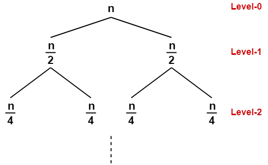
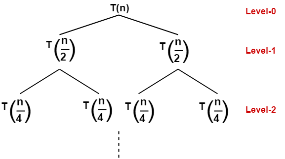
  • A problem of size n will get divided into 2 sub-problems of size n/2.
  • Then, each sub-problem of size n/2 will get divided into 2 sub-problems of size n/4 and so on.
  • At the bottom most layer, the size of sub-problems will reduce to 1.


This is illustrated through following recursion tree-


The given recurrence relation shows-

  • The cost of dividing a problem of size n into its 2 sub-problems and then combining its solution is n.
  • The cost of dividing a problem of size n/2 into its 2 sub-problems and then combining its solution is n/2 and so on.


This is illustrated through following recursion tree where each node represents the cost of the corresponding sub-problem-


Step-02:


Determine cost of each level-

  • Cost of level-0 = n
  • Cost of level-1 = n/2 + n/2 = n
  • Cost of level-2 = n/4 + n/4 + n/4 + n/4 = n and so on.


Step-03:


Determine total number of levels in the recursion tree-

  • Size of sub-problem at level-0 = n/20
  • Size of sub-problem at level-1 = n/21
  • Size of sub-problem at level-2 = n/22


Continuing in similar manner, we have-

Size of sub-problem at level-i = n/2i

Suppose at level-x (last level), size of sub-problem becomes 1. Then-

n / 2x = 1

2x = n

Taking log on both sides, we get-

xlog2 = logn

x = log2n


∴ Total number of levels in the recursion tree = log2n + 1


Step-04:


Determine number of nodes in the last level-

  • Level-0 has 20 nodes i.e. 1 node
  • Level-1 has 21 nodes i.e. 2 nodes
  • Level-2 has 22 nodes i.e. 4 nodes


Continuing in similar manner, we have-

Level-log2n has 2log2n nodes i.e. n nodes


Step-05:


Determine cost of last level-

Cost of last level = n x T(1) = θ(n)


Step-06:


Add costs of all the levels of the recursion tree and simplify the expression so obtained in terms of asymptotic notation-


= n x log2n + θ (n)

= nlog2n + θ (n)

= θ (nlog2n)


Problem-02:


Solve the following recurrence relation using recursion tree method-

T(n) = T(n/5) + T(4n/5) + n


Solution-


Step-01:


Draw a recursion tree based on the given recurrence relation.


The given recurrence relation shows-

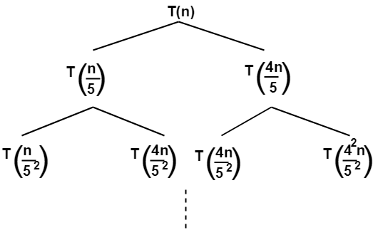
  • A problem of size n will get divided into 2 sub-problems- one of size n/5 and another of size 4n/5.
  • Then, sub-problem of size n/5 will get divided into 2 sub-problems- one of size n/52 and another of size 4n/52.
  • On the other side, sub-problem of size 4n/5 will get divided into 2 sub-problems- one of size 4n/52 and another of size 42n/5and so on.
  • At the bottom most layer, the size of sub-problems will reduce to 1.


This is illustrated through following recursion tree-


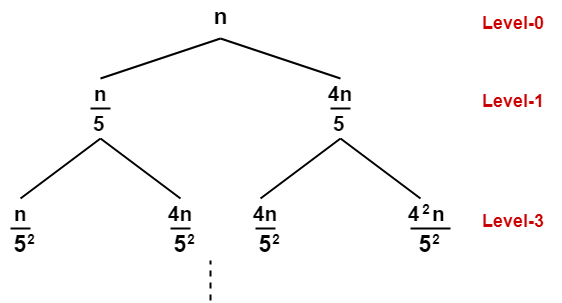
The given recurrence relation shows-

  • The cost of dividing a problem of size n into its 2 sub-problems and then combining its solution is n.
  • The cost of dividing a problem of size n/5 into its 2 sub-problems and then combining its solution is n/5.
  • The cost of dividing a problem of size 4n/5 into its 2 sub-problems and then combining its solution is 4n/5 and so on.


This is illustrated through following recursion tree where each node represents the cost of the corresponding sub-problem-


Step-02:


Determine cost of each level-

  • Cost of level-0 = n
  • Cost of level-1 = n/5 + 4n/5 = n
  • Cost of level-2 = n/52 + 4n/52 + 4n/52 + 42n/52 = n


Step-03:


Determine total number of levels in the recursion tree. We will consider the rightmost sub tree as it goes down to the deepest level-

  • Size of sub-problem at level-0 = (4/5)0n
  • Size of sub-problem at level-1 =(4/5)1n
  • Size of sub-problem at level-2 =(4/5)2n


Continuing in similar manner, we have-

Size of sub-problem at level-i = (4/5)in

Suppose at level-x (last level), size of sub-problem becomes 1. Then-

(4/5)xn = 1

(4/5)x = 1/n

Taking log on both sides, we get-

xlog(4/5) = log(1/n)

x = log5/4n


∴ Total number of levels in the recursion tree = log5/4n + 1


Step-04:


Determine number of nodes in the last level-

  • Level-0 has 20 nodes i.e. 1 node
  • Level-1 has 21 nodes i.e. 2 nodes
  • Level-2 has 22 nodes i.e. 4 nodes


Continuing in similar manner, we have-

Level-log5/4n has 2log5/4n nodes


Step-05:


Determine cost of last level-

Cost of last level = 2log5/4n x T(1) = θ(2log5/4n) = θ(nlog5/42)


Step-06:


Add costs of all the levels of the recursion tree and simplify the expression so obtained in terms of asymptotic notation-


= nlog5/4n + θ(nlog5/42)

= θ(nlog5/4n)


Problem-03:


Solve the following recurrence relation using recursion tree method-

T(n) = 3T(n/4) + cn2


Solution-


Step-01:


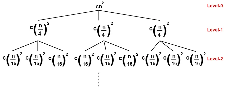
Draw a recursion tree based on the given recurrence relation-


(Here, we have directly drawn a recursion tree representing the cost of sub problems)


Step-02:


Determine cost of each level-

  • Cost of level-0 = cn2
  • Cost of level-1 = c(n/4)2 + c(n/4)+ c(n/4)2 = (3/16)cn2
  • Cost of level-2 = c(n/16)2 x 9 = (9/162)cn2


Step-03:


Determine total number of levels in the recursion tree-

  • Size of sub-problem at level-0 = n/40
  • Size of sub-problem at level-1 = n/41
  • Size of sub-problem at level-2 = n/42


Continuing in similar manner, we have-

Size of sub-problem at level-i = n/4i

Suppose at level-x (last level), size of sub-problem becomes 1. Then-

n/4x = 1

4x = n

Taking log on both sides, we get-

xlog4 = logn

x = log4n


∴ Total number of levels in the recursion tree = log4n + 1


Step-04:


Determine number of nodes in the last level-

  • Level-0 has 30 nodes i.e. 1 node
  • Level-1 has 31 nodes i.e. 3 nodes
  • Level-2 has 32 nodes i.e. 9 nodes


Continuing in similar manner, we have-

Level-log4n has 3log4n nodes i.e. nlog43 nodes


Step-05:


Determine cost of last level-

Cost of last level = nlog43 x T(1) = θ(nlog43)


Step-06:


Add costs of all the levels of the recursion tree and simplify the expression so obtained in terms of asymptotic notation-


= cn2 { 1 + (3/16) + (3/16)2 + ……… } + θ(nlog43)


Now, { 1 + (3/16) + (3/16)2 + ……… } forms an infinite Geometric progression.


On solving, we get-

= (16/13)cn2 { 1 – (3/16)log4n } + θ(nlog43)

= (16/13)cn2 – (16/13)cn2 (3/16)log4n + θ(nlog43)

= O(n2)


To gain better understanding about Recursion Tree,

Watch this Video Lecture


Next Article- DFS Algorithm


Get more notes and other study material of Design and Analysis of Algorithms.

Watch video lectures by visiting our YouTube channel LearnVidFun.