Tag: Machine Learning

Current Research Trends in Machine Learning

Current Research Trends in Machine Learning in Education-
 

Current Research Trends in Machine Learning


Technology plays a crucial role in the lives of everyone. Almost all the functions are automated in every sphere of human activity. It’s done to simplify all the processes, make them run faster, easier, and more productively. Although many people oppose the implementation of technology, its advantages are undeniable. One of the common branches of technology present in education is machine learning. It’s a specific study of algorithms and statistical models that are used by personal computers, laptops, and similar devices. Thanks to those algorithms and statistical models, technological devices can fulfill different tasks and objectives.


Many students prefer to become specialists in this industry, but the learning process is pretty complex for them. Some of them use the assistance of a Cheap Research Paper Writing Service to resolve their impediments by means of professional academic writers. Nonetheless, it’s another question that will be discussed in future posts. In the meanwhile, we’d like to highlight current research trends in machine learning in education and clarify their value for the educational sector.


The Main Developers-


First, we want to outline the main participants in machine learning who will actively collaborate with the system of education. Their devices and applications will determine the effectiveness of the learning process for the next decade or more.

The main role in machine learning for education will play:

  • IBM
  • Microsoft
  • Google
  • Amazon
  • Quantum Adaptive Learning
  • DreamBox Learning
  • Pearson
  • Bridge-U and others


Adoption Of Cloud Technology-


One of the major trends of learning in education is the implementation of Cloud-Based Technology The most important benefit of this kind of technology is to save expenses for educational institutions. It has segmented the entire process of education and simplified it. Students can easily and quickly access the required information in any discipline, fulfill the necessary tasks, and save the results online. This information will never be lost unless users decide to delete it completely.


Digital Assistants-


Although the role of teachers is important, the usefulness of digital assistants offers multiple dividends for all participants of the educational process. Teachers and professors are human, and they cannot devote all their time to their students. In the meanwhile, students frequently have questions when they are already home, and it’s quite late. Thus, a digital assistant comes in handy.


This trend claims that students can resolve their academic complications at any suitable time. Digital assistants are intelligent AI-based (artificial intelligence) machines. They have the knowledge and experience of real educators and can answer most of the questions. For example, a student doesn’t know how to complete an expository essay. The AI-instructor will provide the necessary tips and recommendations, will give resourceful information websites, and something of the kind. Students may receive educational feedback day and night!


Studying Education Market-


Machine learning may propose future development in the educational sector. The technology uses specific algorithms that gather information about education, the objectives of the country’s policy, and the needs of its participants (learners and educators). Afterward, it analyzed this information to propose Clear Insights. It may suggest effective solutions to the current problems and offer new methodologies in the future. For example, it will give predictions for education market dynamics, competition in the field, regional analysis, etc.


Virtual & Augmented Reality-


This research trend is popular and prospective for at least 5 years. The tendency will not decrease in the upcoming decades and its productivity will only increase. This unique technology sufficiently enhances the productivity of the learning process because it ensures a life-like experience. Students can put on special glasses and ear heads to see and listen to a journey into ancient times, see how a manufacturing process runs, or how the surgery is carried out. This practice enhances the interest of students in the educational process.


Online Assessments-


Another crucial trend is important for teachers and professors. It’s an online assessment of students. It’s no secret that educators are overloaded with different responsibilities and duties. They frequently don’t have enough time for academic consultations, help for their students, as well as their private life. Technology can resolve this serious drawback.


Many colleges and universities already use online evaluation of learning results. Smart AI checks and analyzes the results of every lesson, lecture, and test. It summarizes grades instead of educators. It likewise plans future events, creates reasonable schedules, and so on. Thus, teachers and professors can partially get rid of this burden.


Adoption Of Machine Learning-


We want to pay attention to the process of implementation of machine learning in the educational sector. Even if the technology is beneficial and highly efficacious, the wrong use of it will destroy everything. This information will be helpful for educators and educational institutions.


Make allowances for the following recommendations:

  • Set clear objectives- Before an institution implements any technological devices and programs, it’s supposed to clarify objectives for itself to understand how to use technology effectively.
  • Consider finances- The administrations of every school, college, and university should assess their budgets. Technology has its price and every educational institution should be confident that it can afford the implementation of new technology.
  • Stick to realism- The use of technology should be realistic. If the institution doesn’t have enough qualified experts or funds to implement machine learning, it shouldn’t utilize it beforehand.
  • Educate teaching staff- Not all teachers and professors know how to work with new technology. Therefore, every institution is obliged to provide training courses to educate its teaching staff.


If educational institutions take into account these recommendations, they will definitely enjoy success. They will avoid possible delays and complications. Machine learning trends will serve effectively for educators and learners.


It goes beyond all doubts that machine learning is an important industry, and it’s used by education. Thanks to understanding the way certain applications work, educators and learners can implement them to boost the productivity of the learning process. The trends highlighted in our informative article determine the future course of education.
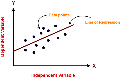
 

Linear Regression Machine Learning | Examples

Linear Regression-


In Machine Learning,

  • Linear Regression is a supervised machine learning algorithm.
  • It tries to find out the best linear relationship that describes the data you have.
  • It assumes that there exists a linear relationship between a dependent variable and independent variable(s).
  • The value of the dependent variable of a linear regression model is a continuous value i.e. real numbers.


Also Read- Machine Learning Algorithms


Representing Linear Regression Model-


Linear regression model represents the linear relationship between a dependent variable and independent variable(s) via a sloped straight line.


The sloped straight line representing the linear relationship that fits the given data best is called as a regression line.

It is also called as best fit line.


Types of Linear Regression-


Based on the number of independent variables, there are two types of linear regression-


  1. Simple Linear Regression
  2. Multiple Linear Regression


1. Simple Linear Regression-


In simple linear regression, the dependent variable depends only on a single independent variable.


For simple linear regression, the form of the model is-

Y = β0 + β1X


Here,

  • Y is a dependent variable.
  • X is an independent variable.
  • β0 and β1 are the regression coefficients.
  • β0 is the intercept or the bias that fixes the offset to a line.
  • β1 is the slope or weight that specifies the factor by which X has an impact on Y.


There are following 3 cases possible-


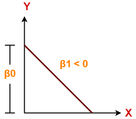
Case-01: β1 < 0


  • It indicates that variable X has negative impact on Y.
  • If X increases, Y will decrease and vice-versa.


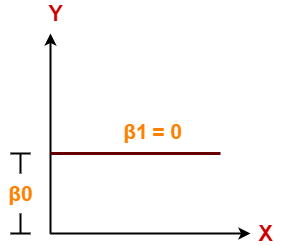
Case-02: β1 = 0


  • It indicates that variable X has no impact on Y.
  • If X changes, there will be no change in Y.


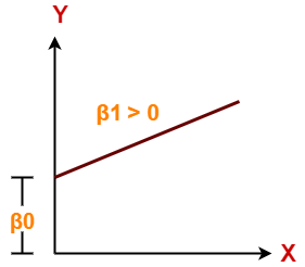
Case-03: β1 > 0


  • It indicates that variable X has positive impact on Y.
  • If X increases, Y will increase and vice-versa.


2. Multiple Linear Regression-


In multiple linear regression, the dependent variable depends on more than one independent variables.


For multiple linear regression, the form of the model is-

Y = β0 + β1X1 + β2X2 + β3X3 + …… + βnXn


Here,

  • Y is a dependent variable.
  • X1, X2, …., Xn are independent variables.
  • β0, β1,…, βn are the regression coefficients.
  • βj (1<=j<=n) is the slope or weight that specifies the factor by which Xj has an impact on Y.


To gain better understanding about Linear Regression,

Watch this Video Lecture


Get more notes and other study material of Machine Learning.

Watch video lectures by visiting our YouTube channel LearnVidFun.

Principal Component Analysis | Dimension Reduction

Dimension Reduction-


In pattern recognition, Dimension Reduction is defined as-

  • It is a process of converting a data set having vast dimensions into a data set with lesser dimensions.
  • It ensures that the converted data set conveys similar information concisely.


Example-


Consider the following example-

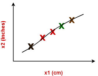
  • The following graph shows two dimensions x1 and x2.
  • x1 represents the measurement of several objects in cm.
  • x2 represents the measurement of several objects in inches.


In machine learning,

  • Using both these dimensions convey similar information.
  • Also, they introduce a lot of noise in the system.
  • So, it is better to use just one dimension.


Using dimension reduction techniques-

  • We convert the dimensions of data from 2 dimensions (x1 and x2) to 1 dimension (z1).
  • It makes the data relatively easier to explain.


Benefits-


Dimension reduction offers several benefits such as-

  • It compresses the data and thus reduces the storage space requirements.
  • It reduces the time required for computation since less dimensions require less computation.
  • It eliminates the redundant features.
  • It improves the model performance.


Dimension Reduction Techniques-


The two popular and well-known dimension reduction techniques are-


  1. Principal Component Analysis (PCA)
  2. Fisher Linear Discriminant Analysis (LDA)


In this article, we will discuss about Principal Component Analysis.


Principal Component Analysis-


  • Principal Component Analysis is a well-known dimension reduction technique.
  • It transforms the variables into a new set of variables called as principal components.
  • These principal components are linear combination of original variables and are orthogonal.
  • The first principal component accounts for most of the possible variation of original data.
  • The second principal component does its best to capture the variance in the data.
  • There can be only two principal components for a two-dimensional data set.


PCA Algorithm-


The steps involved in PCA Algorithm are as follows-


Step-01: Get data.

Step-02: Compute the mean vector (µ).

Step-03: Subtract mean from the given data.

Step-04: Calculate the covariance matrix.

Step-05: Calculate the eigen vectors and eigen values of the covariance matrix.

Step-06: Choosing components and forming a feature vector.

Step-07: Deriving the new data set.


PRACTICE PROBLEMS BASED ON PRINCIPAL COMPONENT ANALYSIS-


Problem-01:


Given data = { 2, 3, 4, 5, 6, 7 ; 1, 5, 3, 6, 7, 8 }.

Compute the principal component using PCA Algorithm.


OR


Consider the two dimensional patterns (2, 1), (3, 5), (4, 3), (5, 6), (6, 7), (7, 8).

Compute the principal component using PCA Algorithm.


OR


Compute the principal component of following data-

CLASS 1

X = 2 , 3 , 4

Y = 1 , 5 , 3

CLASS 2

X = 5 , 6 , 7

Y = 6 , 7 , 8


Solution-


We use the above discussed PCA Algorithm-


Step-01:


Get data.

The given feature vectors are-

  • x1 = (2, 1)
  • x2 = (3, 5)
  • x3 = (4, 3)
  • x4 = (5, 6)
  • x5 = (6, 7)
  • x6 = (7, 8)


Step-02:


Calculate the mean vector (µ).


Mean vector (µ)

= ((2 + 3 + 4 + 5 + 6 + 7) / 6, (1 + 5 + 3 + 6 + 7 + 8) / 6)

= (4.5, 5)


Thus,


Step-03:


Subtract mean vector (µ) from the given feature vectors.

  • x1 – µ = (2 – 4.5, 1 – 5) = (-2.5, -4)
  • x2 – µ = (3 – 4.5, 5 – 5) = (-1.5, 0)
  • x3 – µ = (4 – 4.5, 3 – 5) = (-0.5, -2)
  • x4 – µ = (5 – 4.5, 6 – 5) = (0.5, 1)
  • x5 – µ = (6 – 4.5, 7 – 5) = (1.5, 2)
  • x6 – µ = (7 – 4.5, 8 – 5) = (2.5, 3)


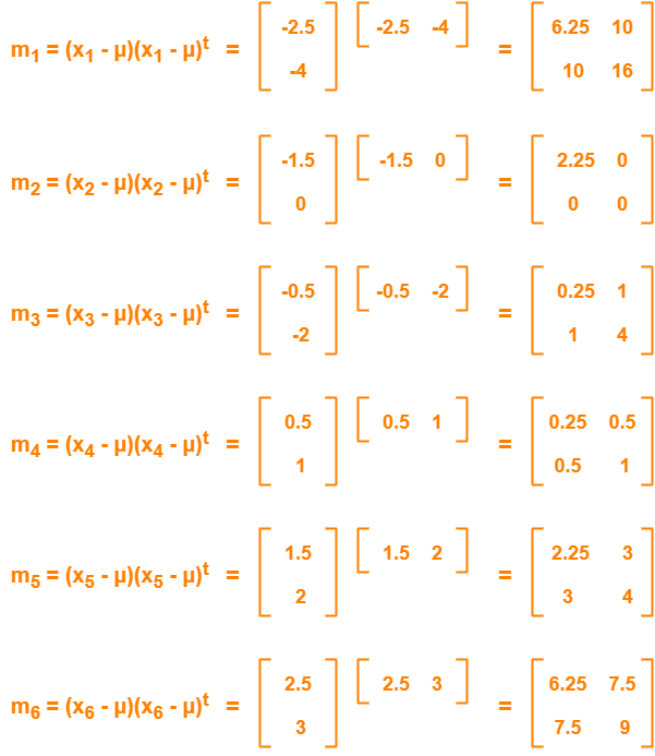
Feature vectors (xi) after subtracting mean vector (µ) are-


Step-04:


Calculate the covariance matrix.

Covariance matrix is given by-


Now,


Now,

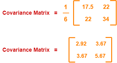
Covariance matrix

= (m1 + m2 + m3 + m4 + m5 + m6) / 6


On adding the above matrices and dividing by 6, we get-


Step-05:


Calculate the eigen values and eigen vectors of the covariance matrix.

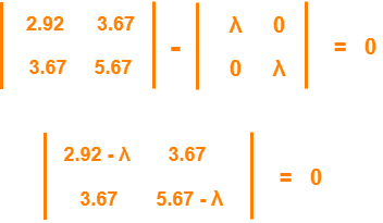
λ is an eigen value for a matrix M if it is a solution of the characteristic equation |M – λI| = 0.

So, we have-


From here,

(2.92 – λ)(5.67 – λ) – (3.67 x 3.67) = 0

16.56 – 2.92λ – 5.67λ + λ2 – 13.47 = 0

λ2 – 8.59λ + 3.09 = 0


Solving this quadratic equation, we get λ = 8.22, 0.38

Thus, two eigen values are λ1 = 8.22 and λ2 = 0.38.


Clearly, the second eigen value is very small compared to the first eigen value.

So, the second eigen vector can be left out.


Eigen vector corresponding to the greatest eigen value is the principal component for the given data set.

So. we find the eigen vector corresponding to eigen value λ1.


We use the following equation to find the eigen vector-

MX = λX

where-

  • M = Covariance Matrix
  • X = Eigen vector
  • λ = Eigen value


Substituting the values in the above equation, we get-


Solving these, we get-

2.92X1 + 3.67X2 = 8.22X1

3.67X1 + 5.67X2 = 8.22X2


On simplification, we get-

5.3X1 = 3.67X2       ………(1)

3.67X1 = 2.55X2     ………(2)


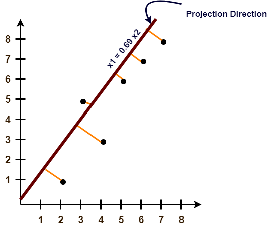
From (1) and (2), X1 = 0.69X2

From (2), the eigen vector is-


Thus, principal component for the given data set is-


Lastly, we project the data points onto the new subspace as-


Problem-02:


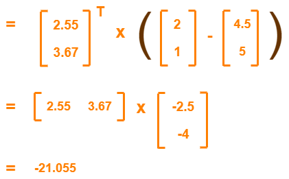
Use PCA Algorithm to transform the pattern (2, 1) onto the eigen vector in the previous question.


Solution-


The given feature vector is (2, 1).


The feature vector gets transformed to

= Transpose of Eigen vector x (Feature Vector – Mean Vector)


To gain better understanding about Principal Component Analysis,

Watch this Video Lecture


Get more notes and other study material of Pattern Recognition.

Watch video lectures by visiting our YouTube channel LearnVidFun.

K-Means Clustering Algorithm | Examples

K-Means Clustering-


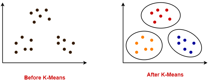
  • K-Means clustering is an unsupervised iterative clustering technique.
  • It partitions the given data set into k predefined distinct clusters.
  • A cluster is defined as a collection of data points exhibiting certain similarities.


It partitions the data set such that-

  • Each data point belongs to a cluster with the nearest mean.
  • Data points belonging to one cluster have high degree of similarity.
  • Data points belonging to different clusters have high degree of dissimilarity.


K-Means Clustering Algorithm-


K-Means Clustering Algorithm involves the following steps-


Step-01:


  • Choose the number of clusters K.


Step-02:


  • Randomly select any K data points as cluster centers.
  • Select cluster centers in such a way that they are as farther as possible from each other.


Step-03:


  • Calculate the distance between each data point and each cluster center.
  • The distance may be calculated either by using given distance function or by using euclidean distance formula.


Step-04:


  • Assign each data point to some cluster.
  • A data point is assigned to that cluster whose center is nearest to that data point.


Step-05:


  • Re-compute the center of newly formed clusters.
  • The center of a cluster is computed by taking mean of all the data points contained in that cluster.


Step-06:


Keep repeating the procedure from Step-03 to Step-05 until any of the following stopping criteria is met-

  • Center of newly formed clusters do not change
  • Data points remain present in the same cluster
  • Maximum number of iterations are reached


Advantages-


K-Means Clustering Algorithm offers the following advantages-


Point-01:


It is relatively efficient with time complexity O(nkt) where-

  • n = number of instances
  • k = number of clusters
  • t = number of iterations


Point-02:


  • It often terminates at local optimum.
  • Techniques such as Simulated Annealing or Genetic Algorithms may be used to find the global optimum.


Disadvantages-


K-Means Clustering Algorithm has the following disadvantages-

  • It requires to specify the number of clusters (k) in advance.
  • It can not handle noisy data and outliers.
  • It is not suitable to identify clusters with non-convex shapes.


PRACTICE PROBLEMS BASED ON K-MEANS CLUSTERING ALGORITHM-


Problem-01:


Cluster the following eight points (with (x, y) representing locations) into three clusters:

A1(2, 10), A2(2, 5), A3(8, 4), A4(5, 8), A5(7, 5), A6(6, 4), A7(1, 2), A8(4, 9)


Initial cluster centers are: A1(2, 10), A4(5, 8) and A7(1, 2).

The distance function between two points a = (x1, y1) and b = (x2, y2) is defined as-

Ρ(a, b) = |x2 – x1| + |y2 – y1|


Use K-Means Algorithm to find the three cluster centers after the second iteration.


Solution-


We follow the above discussed K-Means Clustering Algorithm-


Iteration-01:


  • We calculate the distance of each point from each of the center of the three clusters.
  • The distance is calculated by using the given distance function.


The following illustration shows the calculation of distance between point A1(2, 10) and each of the center of the three clusters-


Calculating Distance Between A1(2, 10) and C1(2, 10)-


Ρ(A1, C1)

= |x2 – x1| + |y2 – y1|

= |2 – 2| + |10 – 10|

= 0


Calculating Distance Between A1(2, 10) and C2(5, 8)-


Ρ(A1, C2)

= |x2 – x1| + |y2 – y1|

= |5 – 2| + |8 – 10|

= 3 + 2

= 5


Calculating Distance Between A1(2, 10) and C3(1, 2)-


Ρ(A1, C3)

= |x2 – x1| + |y2 – y1|

= |1 – 2| + |2 – 10|

= 1 + 8

= 9


In the similar manner, we calculate the distance of other points from each of the center of the three clusters.


Next,

  • We draw a table showing all the results.
  • Using the table, we decide which point belongs to which cluster.
  • The given point belongs to that cluster whose center is nearest to it.


Given Points Distance from center (2, 10) of Cluster-01 Distance from center (5, 8) of Cluster-02 Distance from center (1, 2) of Cluster-03 Point belongs to Cluster
A1(2, 10) 0 5 9 C1
A2(2, 5) 5 6 4 C3
A3(8, 4) 12 7 9 C2
A4(5, 8) 5 0 10 C2
A5(7, 5) 10 5 9 C2
A6(6, 4) 10 5 7 C2
A7(1, 2) 9 10 0 C3
A8(4, 9) 3 2 10 C2


From here, New clusters are-


Cluster-01:


First cluster contains points-

  • A1(2, 10)


Cluster-02:


Second cluster contains points-

  • A3(8, 4)
  • A4(5, 8)
  • A5(7, 5)
  • A6(6, 4)
  • A8(4, 9)


Cluster-03:


Third cluster contains points-

  • A2(2, 5)
  • A7(1, 2)


Now,

  • We re-compute the new cluster clusters.
  • The new cluster center is computed by taking mean of all the points contained in that cluster.


For Cluster-01:


  • We have only one point A1(2, 10) in Cluster-01.
  • So, cluster center remains the same.


For Cluster-02:


Center of Cluster-02

= ((8 + 5 + 7 + 6 + 4)/5, (4 + 8 + 5 + 4 + 9)/5)

= (6, 6)


For Cluster-03:


Center of Cluster-03

= ((2 + 1)/2, (5 + 2)/2)

= (1.5, 3.5)


This is completion of Iteration-01.


Iteration-02:


  • We calculate the distance of each point from each of the center of the three clusters.
  • The distance is calculated by using the given distance function.


The following illustration shows the calculation of distance between point A1(2, 10) and each of the center of the three clusters-


Calculating Distance Between A1(2, 10) and C1(2, 10)-


Ρ(A1, C1)

= |x2 – x1| + |y2 – y1|

= |2 – 2| + |10 – 10|

= 0


Calculating Distance Between A1(2, 10) and C2(6, 6)-


Ρ(A1, C2)

= |x2 – x1| + |y2 – y1|

= |6 – 2| + |6 – 10|

= 4 + 4

= 8


Calculating Distance Between A1(2, 10) and C3(1.5, 3.5)-


Ρ(A1, C3)

= |x2 – x1| + |y2 – y1|

= |1.5 – 2| + |3.5 – 10|

= 0.5 + 6.5

= 7


In the similar manner, we calculate the distance of other points from each of the center of the three clusters.


Next,

  • We draw a table showing all the results.
  • Using the table, we decide which point belongs to which cluster.
  • The given point belongs to that cluster whose center is nearest to it.


Given Points Distance from center (2, 10) of Cluster-01 Distance from center (6, 6) of Cluster-02 Distance from center (1.5, 3.5) of Cluster-03 Point belongs to Cluster
A1(2, 10) 0 8 7 C1
A2(2, 5) 5 5 2 C3
A3(8, 4) 12 4 7 C2
A4(5, 8) 5 3 8 C2
A5(7, 5) 10 2 7 C2
A6(6, 4) 10 2 5 C2
A7(1, 2) 9 9 2 C3
A8(4, 9) 3 5 8 C1


From here, New clusters are-


Cluster-01:


First cluster contains points-

  • A1(2, 10)
  • A8(4, 9)


Cluster-02:


Second cluster contains points-

  • A3(8, 4)
  • A4(5, 8)
  • A5(7, 5)
  • A6(6, 4)


Cluster-03:


Third cluster contains points-

  • A2(2, 5)
  • A7(1, 2)


Now,

  • We re-compute the new cluster clusters.
  • The new cluster center is computed by taking mean of all the points contained in that cluster.


For Cluster-01:


Center of Cluster-01

= ((2 + 4)/2, (10 + 9)/2)

= (3, 9.5)


For Cluster-02:


Center of Cluster-02

= ((8 + 5 + 7 + 6)/4, (4 + 8 + 5 + 4)/4)

= (6.5, 5.25)


For Cluster-03:


Center of Cluster-03

= ((2 + 1)/2, (5 + 2)/2)

= (1.5, 3.5)


This is completion of Iteration-02.


After second iteration, the center of the three clusters are-

  • C1(3, 9.5)
  • C2(6.5, 5.25)
  • C3(1.5, 3.5)


Problem-02:


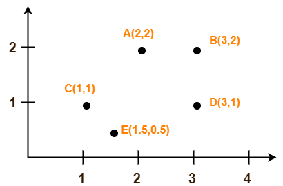
Use K-Means Algorithm to create two clusters-


Solution-


We follow the above discussed K-Means Clustering Algorithm.

Assume A(2, 2) and C(1, 1) are centers of the two clusters.


Iteration-01:


  • We calculate the distance of each point from each of the center of the two clusters.
  • The distance is calculated by using the euclidean distance formula.


The following illustration shows the calculation of distance between point A(2, 2) and each of the center of the two clusters-


Calculating Distance Between A(2, 2) and C1(2, 2)-


Ρ(A, C1)

= sqrt [ (x2 – x1)2 + (y2 – y1)2 ]

= sqrt [ (2 – 2)2 + (2 – 2)2 ]

= sqrt [ 0 + 0 ]

= 0


Calculating Distance Between A(2, 2) and C2(1, 1)-


Ρ(A, C2)

= sqrt [ (x2 – x1)2 + (y2 – y1)2 ]

= sqrt [ (1 – 2)2 + (1 – 2)2 ]

= sqrt [ 1 + 1 ]

= sqrt [ 2 ]

= 1.41


In the similar manner, we calculate the distance of other points from each of the center of the two clusters.


Next,

  • We draw a table showing all the results.
  • Using the table, we decide which point belongs to which cluster.
  • The given point belongs to that cluster whose center is nearest to it.


Given Points Distance from center (2, 2) of Cluster-01 Distance from center (1, 1) of Cluster-02 Point belongs to Cluster
A(2, 2) 0 1.41 C1
B(3, 2) 1 2.24 C1
C(1, 1) 1.41 0 C2
D(3, 1) 1.41 2 C1
E(1.5, 0.5) 1.58 0.71 C2


From here, New clusters are-


Cluster-01:


First cluster contains points-

  • A(2, 2)
  • B(3, 2)
  • E(1.5, 0.5)
  • D(3, 1)


Cluster-02:


Second cluster contains points-

  • C(1, 1)
  • E(1.5, 0.5)


Now,

  • We re-compute the new cluster clusters.
  • The new cluster center is computed by taking mean of all the points contained in that cluster.


For Cluster-01:


Center of Cluster-01

= ((2 + 3 + 3)/3, (2 + 2 + 1)/3)

= (2.67, 1.67)


For Cluster-02:


Center of Cluster-02

= ((1 + 1.5)/2, (1 + 0.5)/2)

= (1.25, 0.75)


This is completion of Iteration-01.

Next, we go to iteration-02, iteration-03 and so on until the centers do not change anymore.


To gain better understanding about K-Means Clustering Algorithm,

Watch this Video Lecture


Next Article- Principal Component Analysis


Get more notes and other study material of Pattern Recognition.

Watch video lectures by visiting our YouTube channel LearnVidFun.

Machine Learning Workflow | Process Steps

Machine Learning-


Before you go through this article, make sure that you have gone through the previous article on Machine Learning.


We have discussed-

  • Machine learning is building machines that can adapt and learn from experience.
  • Machine learning systems are not explicitly programmed.


In this article, we will discuss machine learning workflow.


Machine Learning Workflow-


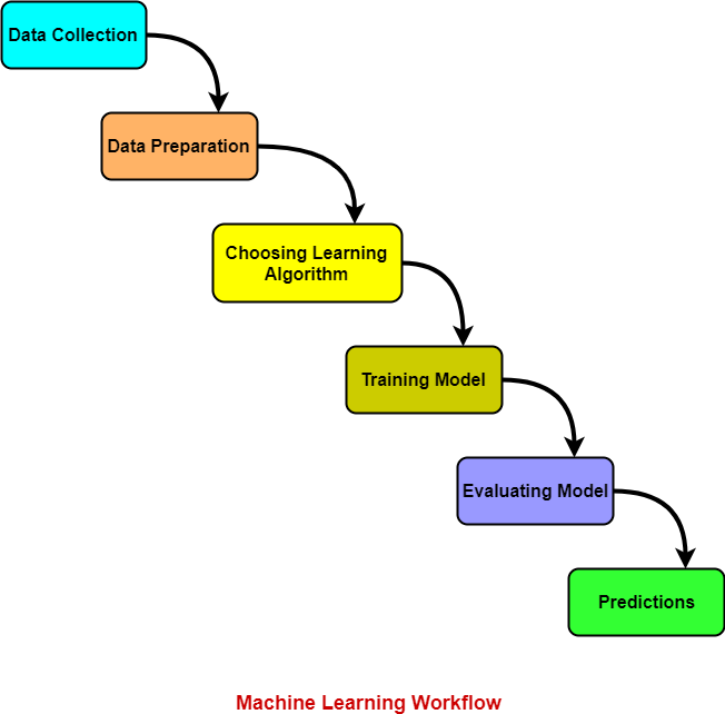
Machine learning workflow refers to the series of stages or steps involved in the process of building a successful machine learning system.


The various stages involved in the machine learning workflow are-


  1. Data Collection
  2. Data Preparation
  3. Choosing Learning Algorithm
  4. Training Model
  5. Evaluating Model
  6. Predictions


Let us discuss each stage one by one.


1. Data Collection-


In this stage,

  • Data is collected from different sources.
  • The type of data collected depends upon the type of desired project.
  • Data may be collected from various sources such as files, databases etc.
  • The quality and quantity of gathered data directly affects the accuracy of the desired system.


2. Data Preparation-


In this stage,

  • Data preparation is done to clean the raw data.
  • Data collected from the real world is transformed to a clean dataset.
  • Raw data may contain missing values, inconsistent values, duplicate instances etc.
  • So, raw data cannot be directly used for building a model.


Different methods of cleaning the dataset are-

  • Ignoring the missing values
  • Removing instances having missing values from the dataset.
  • Estimating the missing values of instances using mean, median or mode.
  • Removing duplicate instances from the dataset.
  • Normalizing the data in the dataset.


This is the most time consuming stage in machine learning workflow.


3. Choosing Learning Algorithm-


In this stage,

  • The best performing learning algorithm is researched.
  • It depends upon the type of problem that needs to solved and the type of data we have.
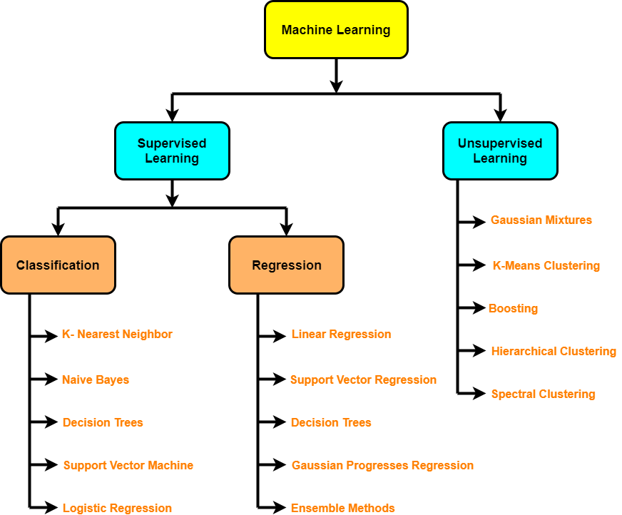
  • If the problem is to classify and the data is labeled, classification algorithms are used.
  • If the problem is to perform a regression task and the data is labeled, regression algorithms are used.
  • If the problem is to create clusters and the data is unlabeled, clustering algorithms are used.


The following chart provides the overview of learning algorithms-


4. Training Model-


In this stage,

  • The model is trained to improve its ability.
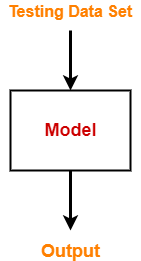
  • The dataset is divided into training dataset and testing dataset.
  • The training and testing split is order of 80/20 or 70/30.
  • It also depends upon the size of the dataset.
  • Training dataset is used for training purpose.
  • Testing dataset is used for the testing purpose.
  • Training dataset is fed to the learning algorithm.
  • The learning algorithm finds a mapping between the input and the output and generates the model.


5. Evaluating Model-


In this stage,

  • The model is evaluated to test if the model is any good.
  • The model is evaluated using the kept-aside testing dataset.
  • It allows to test the model against data that has never been used before for training.
  • Metrics such as accuracy, precision, recall etc are used to test the performance.
  • If the model does not perform well, the model is re-built using different hyper parameters.
  • The accuracy may be further improved by tuning the hyper parameters.


6. Predictions-


In this stage,

  • The built system is finally used to do something useful in the real world.
  • Here, the true value of machine learning is realized.


To gain better understanding about Machine Learning Workflow,

Watch this Video Lecture


Next Article- Linear Regression


Get more notes and other study material of Machine Learning.

Watch video lectures by visiting our YouTube channel LearnVidFun.