Tag: Sorting Algorithms Explained

Bubble Sort Algorithm | Example | Time Complexity

Bubble Sort-


  • Bubble sort is the easiest sorting algorithm to implement.
  • It is inspired by observing the behavior of air bubbles over foam.
  • It is an in-place sorting algorithm.
  • It uses no auxiliary data structures (extra space) while sorting.


How Bubble Sort Works?


  • Bubble sort uses multiple passes (scans) through an array.
  • In each pass, bubble sort compares the adjacent elements of the array.
  • It then swaps the two elements if they are in the wrong order.
  • In each pass, bubble sort places the next largest element to its proper position.
  • In short, it bubbles down the largest element to its correct position.


Bubble Sort Algorithm-


The bubble sort algorithm is given below-


for(int pass=1 ; pass<=n-1 ; ++pass)     // Making passes through array
{
    for(int i=0 ; i<=n-2 ; ++i)
    {
        if(A[i] > A[i+1])                // If adjacent elements are in wrong order
            swap(i,i+1,A);               // Swap them
    }
}

//swap function : Exchange elements from array A at position x,y

void swap(int x, int y, int[] A)
{
    int temp = A[x];
    A[x] = A[y];
    A[y] = temp;
    return ;
}

// pass : Variable to count the number of passes that are done till now
// n : Size of the array
// i : Variable to traverse the array A
// swap() : Function to swap two numbers from the array
// x,y : Indices of the array that needs to be swapped


Bubble Sort Example-


Consider the following array A-


Now, we shall implement the above bubble sort algorithm on this array.


Step-01:


  • We have pass=1 and i=0.
  • We perform the comparison A[0] > A[1] and swaps if the 0th element is greater than the 1th element.
  • Since 6 > 2, so we swap the two elements.


Step-02:


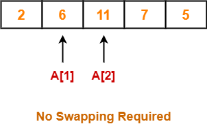
  • We have pass=1 and i=1.
  • We perform the comparison A[1] > A[2] and swaps if the 1th element is greater than the 2th element.
  • Since 6 < 11, so no swapping is required.


Step-03:


  • We have pass=1 and i=2.
  • We perform the comparison A[2] > A[3] and swaps if the 2nd element is greater than the 3rd element.
  • Since 11 > 7, so we swap the two elements.


Step-04:


  • We have pass=1 and i=3.
  • We perform the comparison A[3] > A[4] and swaps if the 3rd element is greater than the 4th element.
  • Since 11 > 5, so we swap the two elements.


Finally after the first pass, we see that the largest element 11 reaches its correct position.


Step-05:


  • Similarly after pass=2, element 7 reaches its correct position.
  • The modified array after pass=2 is shown below-


Step-06:


  • Similarly after pass=3, element 6 reaches its correct position.
  • The modified array after pass=3 is shown below-


Step-07:


  • No further improvement is done in pass=4.
  • This is because at this point, elements 2 and 5 are already present at their correct positions.
  • The loop terminates after pass=4.
  • Finally, the array after pass=4 is shown below-


Optimization Of Bubble Sort Algorithm-


  • If the array gets sorted after a few passes like one or two, then ideally the algorithm should terminate.
  • But still the above algorithm executes the remaining passes which costs extra comparisons.


Optimized Bubble Sort Algorithm-


The optimized bubble sort algorithm is shown below-


for (int pass=1 ; pass<=n-1 ; ++pass)
{
    flag=0                                // flag denotes are there any swaps done in pass

    for (int i=0 ; i<=n-2 ; ++i)
    {
        if(A[i] > A[i+1])
        {
            swap(i,i+1,A);
            flag=1                        // After swap, set flag to 1
        }
    }

    if(flag == 0) break;                  // No swaps indicates we can terminate loop
}

void swap(int x, int y, int[] A)
{
    int temp = A[x];
    A[x] = A[y];
    A[y] = temp;
    return;
}


Explanation-


  • To avoid extra comparisons, we maintain a flag variable.
  • The flag variable helps to break the outer loop of passes after obtaining the sorted array.
  • The initial value of the flag variable is set to 0.
  • The zero value of flag variable denotes that we have not encountered any swaps.
  • Once we need to swap adjacent values for correcting their wrong order, the value of flag variable is set to 1.
  • If we encounter a pass where flag == 0, then it is safe to break the outer loop and declare the array is sorted.


Time Complexity Analysis-


  • Bubble sort uses two loops- inner loop and outer loop.
  • The inner loop deterministically performs O(n) comparisons.


Worst Case-


  • In worst case, the outer loop runs O(n) times.
  • Hence, the worst case time complexity of bubble sort is O(n x n) = O(n2).


Best Case-


  • In best case, the array is already sorted but still to check, bubble sort performs O(n) comparisons.
  • Hence, the best case time complexity of bubble sort is O(n).


Average Case-


  • In average case, bubble sort may require (n/2) passes and O(n) comparisons for each pass.
  • Hence, the average case time complexity of bubble sort is O(n/2 x n) = Θ(n2).


The following table summarizes the time complexities of bubble sort in each case-


Time Complexity
Best Case O(n)
Average Case Θ(n2)
Worst Case O(n2)


From here, it is clear that bubble sort is not at all efficient in terms of time complexity of its algorithm.


Space Complexity Analysis-


  • Bubble sort uses only a constant amount of extra space for variables like flag, i, n.
  • Hence, the space complexity of bubble sort is O(1).
  • It is an in-place sorting algorithm i.e. it modifies elements of the original array to sort the given array.


Properties-


Some of the important properties of bubble sort algorithm are-

  • Bubble sort is a stable sorting algorithm.
  • Bubble sort is an in-place sorting algorithm.
  • The worst case time complexity of bubble sort algorithm is O(n2).
  • The space complexity of bubble sort algorithm is O(1).
  • Number of swaps in bubble sort = Number of inversion pairs present in the given array.
  • Bubble sort is beneficial when array elements are less and the array is nearly sorted.


PRACTICE PROBLEMS BASED ON MERGE SORT ALGORITHM-


Problem-01:


The number of swapping needed to sort the numbers 8, 22, 7, 9, 31, 5, 13 in ascending order using bubble sort is-  (ISRO CS 2017)

  1. 11
  2. 12
  3. 13
  4. 10


Solution-


In bubble sort, Number of swaps required = Number of inversion pairs.

Here, there are 10 inversion pairs present which are-

  1. (8,7)
  2. (22,7)
  3. (22,9)
  4. (8,5)
  5. (22,5)
  6. (7,5)
  7. (9,5)
  8. (31,5)
  9. (22,13)
  10. (31,13)


Thus, Option (D) is correct.


Problem-02:


When will bubble sort take worst-case time complexity?

  1. The array is sorted in ascending order.
  2. The array is sorted in descending order.
  3. Only the first half of the array is sorted.
  4. Only the second half of the array is sorted.


Solution-


  • In bubble sort, Number of swaps required = Number of inversion pairs.
  • When an array is sorted in descending order, the number of inversion pairs = n(n-1)/2 which is maximum for any permutation of array.


Thus, Option (B) is correct.


To gain better understanding about Bubble Sort Algorithm,

Watch this Video Lecture


Next Article- Insertion Sort


Other Popular Sorting Algorithms-


Get more notes and other study material of Design and Analysis of Algorithms.

Watch video lectures by visiting our YouTube channel LearnVidFun.

Merge Sort Algorithm | Example | Time Complexity

Merge Sort-


  • Merge sort is a famous sorting algorithm.
  • It uses a divide and conquer paradigm for sorting.
  • It divides the problem into sub problems and solves them individually.
  • It then combines the results of sub problems to get the solution of the original problem.


How Merge Sort Works?


Before learning how merge sort works, let us learn about the merge procedure of merge sort algorithm.

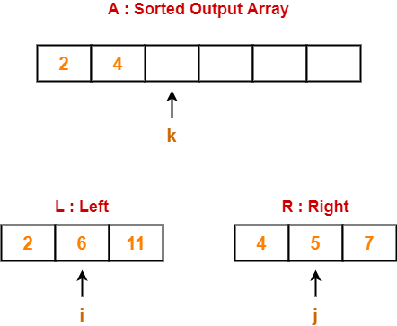
The merge procedure of merge sort algorithm is used to merge two sorted arrays into a third array in sorted order.


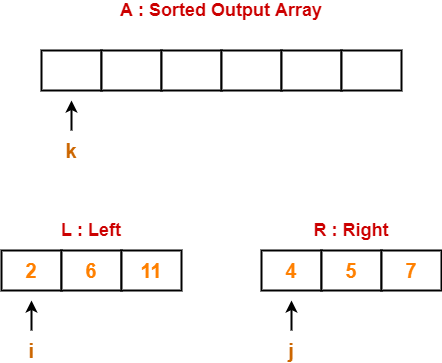
Consider we want to merge the following two sorted sub arrays into a third array in sorted order-


The merge procedure of merge sort algorithm is given below-


// L : Left Sub Array , R : Right Sub Array , A : Array

merge(L, R, A)
{
    nL = length(L)    // Size of Left Sub Array
    nR = length(R)    // Size of Right Sub Array

    i = j = k = 0

    while(i<nL && j<nR)
    {
      /* When both i and j are valid i.e. when both the sub arrays have elements to insert in A */
      
       if(L[i] <= R[j])
       {
          A[k] = L[i]
          k = k+1
          i = i+1
       }
       else
       {
          A[k] = R[j]
          k = k+1
          j = j+1
       }
    }

    // Adding Remaining elements from left sub array to array A
    while(i<nL)
    {
       A[k] = L[i]
       i = i+1
       k = k+1
    }

    // Adding Remaining elements from right sub array to array A
    while(j<nR)
    {
       A[k] = R[j]
       j = j+1
       k = k+1
    }
}


The above merge procedure of merge sort algorithm is explained in the following steps-


Step-01:


  • Create two variables i and j for left and right sub arrays.
  • Create variable k for sorted output array.


Step-02:


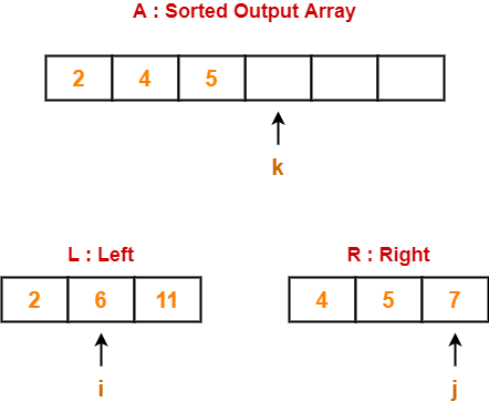
  • We have i = 0, j = 0, k = 0.
  • Since L[0] < R[0], so we perform A[0] = L[0] i.e. we copy the first element from left sub array to our sorted output array.
  • Then, we increment i and k by 1.


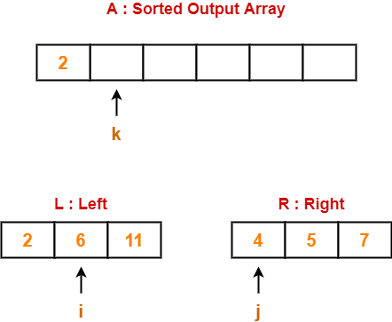
Then, we have-


Step-03:


  • We have i = 1, j = 0, k = 1.
  • Since L[1] > R[0], so we perform A[1] = R[0] i.e. we copy the first element from right sub array to our sorted output array.
  • Then, we increment j and k by 1.


Then, we have-


Step-04:


  • We have i = 1, j = 1, k = 2.
  • Since L[1] > R[1], so we perform A[2] = R[1].
  • Then, we increment j and k by 1.


Then, we have-


Step-05:


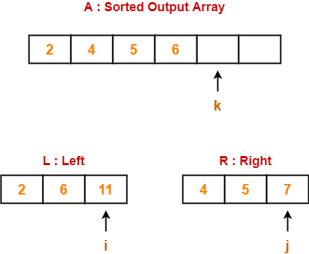
  • We have i = 1, j = 2, k = 3.
  • Since L[1] < R[2], so we perform A[3] = L[1].
  • Then, we increment i and k by 1.


Then, we have-


Step-06:


  • We have i = 2, j = 2, k = 4.
  • Since L[2] > R[2], so we perform A[4] = R[2].
  • Then, we increment j and k by 1.


Then, we have-


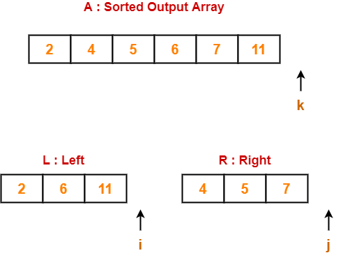
Step-07:


  • Clearly, all the elements from right sub array have been added to the sorted output array.
  • So, we exit the first while loop with the condition while(i<nL && j<nR) since now j>nR.
  • Then, we add remaining elements from the left sub array to the sorted output array using next while loop.


Finally, our sorted output array is-


Basically,

  • After finishing elements from any of the sub arrays, we can add the remaining elements from the other sub array to our sorted output array as it is.
  • This is because left and right sub arrays are already sorted.


Time Complexity

The above mentioned merge procedure takes Θ(n) time.

This is because we are just filling an array of size n from left & right sub arrays by incrementing i and j at most Θ(n) times.


Merge Sort Algorithm-


Merge Sort Algorithm works in the following steps-

  • It divides the given unsorted array into two halves- left and right sub arrays.
  • The sub arrays are divided recursively.
  • This division continues until the size of each sub array becomes 1.
  • After each sub array contains only a single element, each sub array is sorted trivially.
  • Then, the above discussed merge procedure is called.
  • The merge procedure combines these trivially sorted arrays to produce a final sorted array.


The division procedure of merge sort algorithm which uses recursion is given below-


// A : Array that needs to be sorted

MergeSort(A)
{
   n = length(A)
   if n<2 return
   mid = n/2
   left = new_array_of_size(mid)       // Creating temporary array for left
   right = new_array_of_size(n-mid)    // and right sub arrays

   for(int i=0 ; i<=mid-1 ; ++i)
   {
      left[i] = A[i]                  // Copying elements from A to left
   }

   for(int i=mid ; i<=n-1 ; ++i)
   {
      right[i-mid] = A[i]             // Copying elements from A to right
   }

   MergeSort(left)                    // Recursively solving for left sub array
   MergeSort(right)                   // Recursively solving for right sub array

   merge(left, right, A)              // Merging two sorted left/right sub array to final array
}


Merge Sort Example-


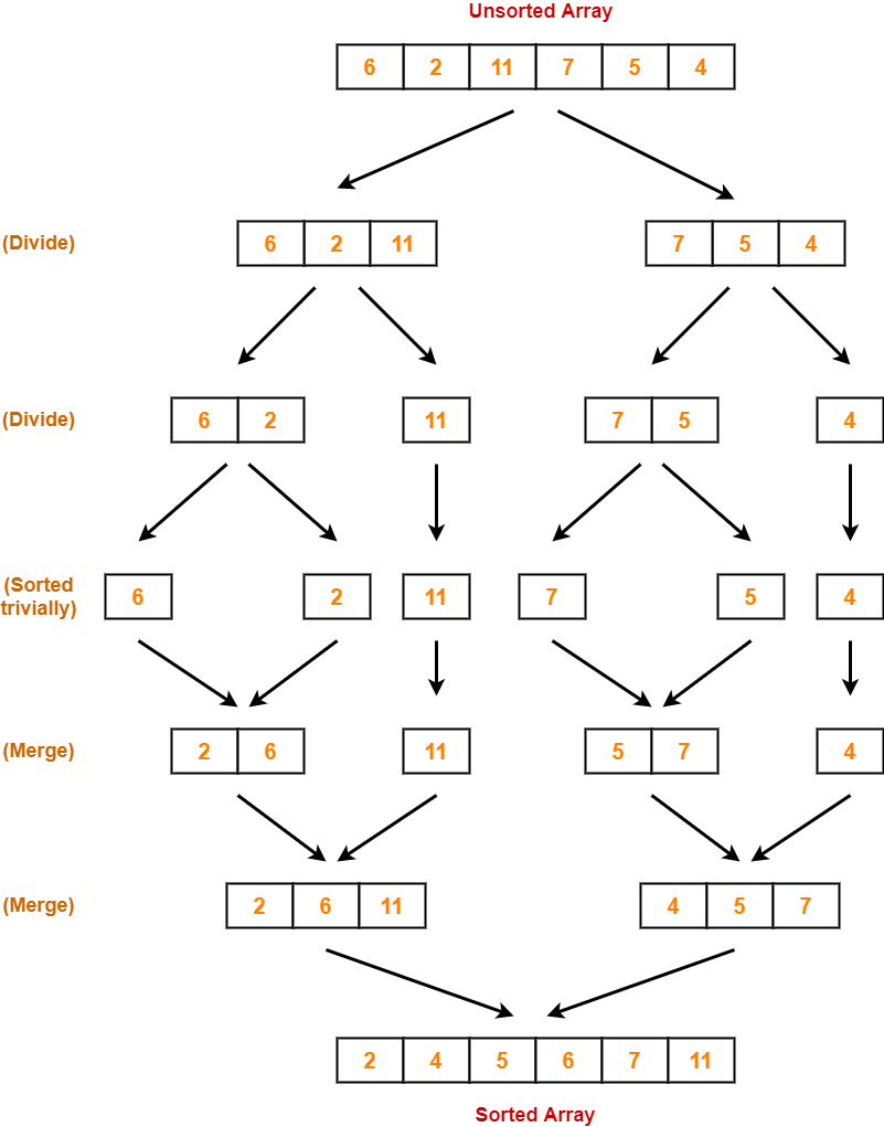
Consider the following elements have to be sorted in ascending order-

6, 2, 11, 7, 5, 4


The merge sort algorithm works as-


Time Complexity Analysis-


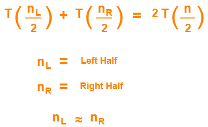
In merge sort, we divide the array into two (nearly) equal halves and solve them recursively using merge sort only.

So, we have-


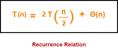
Finally, we merge these two sub arrays using merge procedure which takes Θ(n) time as explained above.


If T(n) is the time required by merge sort for sorting an array of size n, then the recurrence relation for time complexity of merge sort is-


On solving this recurrence relation, we get T(n) = Θ(nlogn).

Thus, time complexity of merge sort algorithm is T(n) = Θ(nlogn).


Also Read- Master’s Theorem for Solving Recurrence Relations


Space Complexity Analysis-


  • Merge sort uses additional memory for left and right sub arrays.
  • Hence, total Θ(n) extra memory is needed.


Properties-


Some of the important properties of merge sort algorithm are-

  • Merge sort uses a divide and conquer paradigm for sorting.
  • Merge sort is a recursive sorting algorithm.
  • Merge sort is a stable sorting algorithm.
  • Merge sort is not an in-place sorting algorithm.
  • The time complexity of merge sort algorithm is Θ(nlogn).
  • The space complexity of merge sort algorithm is Θ(n).


NOTE

Merge sort is the best sorting algorithm in terms of time complexity Θ(nlogn)

if we are not concerned with auxiliary space used.


PRACTICE PROBLEMS BASED ON MERGE SORT ALGORITHM-


Problem-


Assume that a merge sort algorithm in the worst case takes 30 seconds for an input of size 64. Which of the following most closely approximates the maximum input size of a problem that can be solved in 6 minutes? (GATE 2015)

  1. 256
  2. 512
  3. 1024
  4. 2048


Solution-


We know, time complexity of merge sort algorithm is Θ(nlogn).


Step-01:


It is given that a merge sort algorithm in the worst case takes 30 seconds for an input of size 64.

So, we have-


k x nlogn = 30                   (for n = 64)

k x 64 log64 = 30

k x 64 x 6 = 30

From here, k = 5 / 64.


Step-02:


Let n be the maximum input size of a problem that can be solved in 6 minutes (or 360 seconds).

Then, we have-


k x nlogn = 360

(5/64) x nlogn = 360         { Using Result of Step-01 }

nlogn = 72 x 64

nlogn = 4608

On solving this equation, we get n = 512.


Thus, correct option is (B).


To gain better understanding about Merge Sort Algorithm,

Watch this Video Lecture


Next Article- Quick Sort


Other Popular Sorting Algorithms-


Get more notes and other study material of Design and Analysis of Algorithms.

Watch video lectures by visiting our YouTube channel LearnVidFun.
Insertion Sort Algorithm | Example | Time Complexity

Insertion Sort-


  • Insertion sort is an in-place sorting algorithm.
  • It uses no auxiliary data structures while sorting.
  • It is inspired from the way in which we sort playing cards.


How Insertion Sort Works?


Consider the following elements are to be sorted in ascending order-

6, 2, 11, 7, 5


Insertion sort works as-


Firstly,

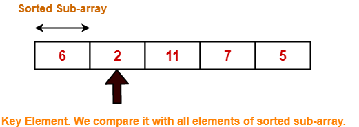
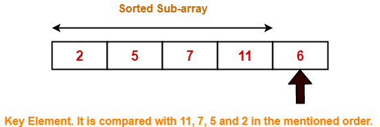
  • It selects the second element (2).
  • It checks whether it is smaller than any of the elements before it.
  • Since 2 < 6, so it shifts 6 towards right and places 2 before it.
  • The resulting list is 2, 6, 11, 7, 5.


Secondly,

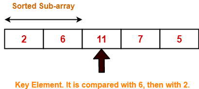
  • It selects the third element (11).
  • It checks whether it is smaller than any of the elements before it.
  • Since 11 > (2, 6), so no shifting takes place.
  • The resulting list remains the same.


Thirdly,

  • It selects the fourth element (7).
  • It checks whether it is smaller than any of the elements before it.
  • Since 7 < 11, so it shifts 11 towards right and places 7 before it.
  • The resulting list is 2, 6, 7, 11, 5.


Fourthly,

  • It selects the fifth element (5).
  • It checks whether it is smaller than any of the elements before it.
  • Since 5 < (6, 7, 11), so it shifts (6, 7, 11) towards right and places 5 before them.
  • The resulting list is 2, 5, 6, 7, 11.


As a result, sorted elements in ascending order are-

2, 5, 6, 7, 11


Insertion Sort Algorithm-


Let A be an array with n elements. The insertion sort algorithm used for sorting is as follows-


for (i = 1 ; i < n ; i++)

{

   key = A [ i ];

   j = i - 1;

   while(j > 0 && A [ j ] > key)

   {

       A [ j+1 ] = A [ j ];

       j--;

    }

    A [ j+1 ] = key;

}


Here,

  • i = variable to traverse the array A
  • key = variable to store the new number to be inserted into the sorted sub-array
  • j = variable to traverse the sorted sub-array


Insertion Sort Example-


Consider the following elements are to be sorted in ascending order-

6, 2, 11, 7, 5


The above insertion sort algorithm works as illustrated below-


Step-01: For i = 1


Step-02: For i = 2


Step-03: For i = 3


2 5 11 7 6 For j = 2; 11 > 7 so A[3] = 11
2 5 11 11 6 For j = 1; 5 < 7 so loop stops and A[2] = 7
2 5 7 11 6 After inner loop ends


Working of inner loop when i = 3


Step-04: For i = 4


Loop gets terminated as ‘i’ becomes 5. The state of array after the loops are finished-


With each loop cycle,

  • One element is placed at the correct location in the sorted sub-array until array A is completely sorted.


Time Complexity Analysis-


  • Selection sort algorithm consists of two nested loops.
  • Owing to the two nested loops, it has O(n2) time complexity.


Time Complexity
Best Case n
Average Case n2
Worst Case n2


Space Complexity Analysis-


  • Selection sort is an in-place algorithm.
  • It performs all computation in the original array and no other array is used.
  • Hence, the space complexity works out to be O(1).


Important Notes-


  • Insertion sort is not a very efficient algorithm when data sets are large.
  • This is indicated by the average and worst case complexities.
  • Insertion sort is adaptive and number of comparisons are less if array is partially sorted.


To gain better understanding about Insertion Sort Algorithm,

Watch this Video Lecture


Next Article- Merge Sort


Other Popular Sorting Algorithms-


Get more notes and other study material of Design and Analysis of Algorithms.

Watch video lectures by visiting our YouTube channel LearnVidFun.
Selection Sort Algorithm | Example | Time Complexity

Selection Sort-


  • Selection sort is one of the easiest approaches to sorting.
  • It is inspired from the way in which we sort things out in day to day life.
  • It is an in-place sorting algorithm because it uses no auxiliary data structures while sorting.


How Selection Sort Works?


Consider the following elements are to be sorted in ascending order using selection sort-

6, 2, 11, 7, 5


Selection sort works as-

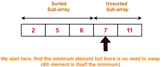
  • It finds the first smallest element (2).
  • It swaps it with the first element of the unordered list.
  • It finds the second smallest element (5).
  • It swaps it with the second element of the unordered list.
  • Similarly, it continues to sort the given elements.


As a result, sorted elements in ascending order are-

2, 5, 6, 7, 11


Selection Sort Algorithm-


Let A be an array with n elements. Then, selection sort algorithm used for sorting is as follows-


for (i = 0 ; i < n-1 ; i++)

{

   index = i;

   for(j = i+1 ; j < n ; j++)

   {

      if(A[j] < A[index])

      index = j;

   }

   temp = A[i];

   A[i] = A[index];

   A[index] = temp;

}


Here,

  • i = variable to traverse the array A
  • index = variable to store the index of minimum element
  • j = variable to traverse the unsorted sub-array
  • temp = temporary variable used for swapping


Selection Sort Example-


Consider the following elements are to be sorted in ascending order-

6, 2, 11, 7, 5


The above selection sort algorithm works as illustrated below-


Step-01: For i = 0


Step-02: For i = 1


Step-03: For i = 2


Step-04: For i = 3


Step-05: For i = 4


Loop gets terminated as ‘i’ becomes 4.


The state of array after the loops are finished is as shown-


With each loop cycle,

  • The minimum element in unsorted sub-array is selected.
  • It is then placed at the correct location in the sorted sub-array until array A is completely sorted.


Time Complexity Analysis-


  • Selection sort algorithm consists of two nested loops.
  • Owing to the two nested loops, it has O(n2) time complexity.


Time Complexity
Best Case n2
Average Case n2
Worst Case n2


Space Complexity Analysis-


  • Selection sort is an in-place algorithm.
  • It performs all computation in the original array and no other array is used.
  • Hence, the space complexity works out to be O(1).


Important Notes-


  • Selection sort is not a very efficient algorithm when data sets are large.
  • This is indicated by the average and worst case complexities.
  • Selection sort uses minimum number of swap operations O(n) among all the sorting algorithms.


To gain better understanding about Selection Sort Algorithm,

Watch this Video Lecture


Next Article- Bubble Sort


Other Popular Sorting Algorithms-


Get more notes and other study material of Design and Analysis of Algorithms.

Watch video lectures by visiting our YouTube channel LearnVidFun.
Topological Sort | Topological Sort Examples

Topological Sort-


Topological Sort is a linear ordering of the vertices in such a way that

if there is an edge in the DAG going from vertex ‘u’ to vertex ‘v’,

then ‘u’ comes before ‘v’ in the ordering.


It is important to note that-

  • Topological Sorting is possible if and only if the graph is a Directed Acyclic Graph.
  • There may exist multiple different topological orderings for a given directed acyclic graph.


Topological Sort Example-


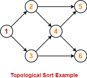
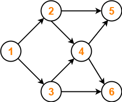
Consider the following directed acyclic graph-


For this graph, following 4 different topological orderings are possible-

  • 1 2 3 4 5 6
  • 1 2 3 4 6 5
  • 1 3 2 4 5 6
  • 1 3 2 4 6 5


Applications of Topological Sort-


Few important applications of topological sort are-

  • Scheduling jobs from the given dependencies among jobs
  • Instruction Scheduling
  • Determining the order of compilation tasks to perform in makefiles
  • Data Serialization


PRACTICE PROBLEMS BASED ON TOPOLOGICAL SORT-


Problem-01:


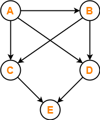
Find the number of different topological orderings possible for the given graph-


Solution-


The topological orderings of the above graph are found in the following steps-


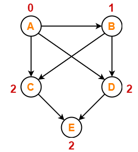
Step-01:


Write in-degree of each vertex-


Step-02:


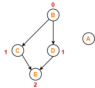
  • Vertex-A has the least in-degree.
  • So, remove vertex-A and its associated edges.
  • Now, update the in-degree of other vertices.


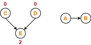
Step-03:


  • Vertex-B has the least in-degree.
  • So, remove vertex-B and its associated edges.
  • Now, update the in-degree of other vertices.


Step-04:


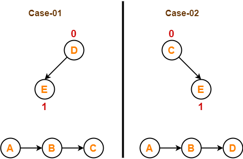
There are two vertices with the least in-degree. So, following 2 cases are possible-


In case-01,

  • Remove vertex-C and its associated edges.
  • Then, update the in-degree of other vertices.


In case-02,

  • Remove vertex-D and its associated edges.
  • Then, update the in-degree of other vertices.


Step-05:


Now, the above two cases are continued separately in the similar manner.


In case-01,

  • Remove vertex-D since it has the least in-degree.
  • Then, remove the remaining vertex-E.


In case-02,

  • Remove vertex-C since it has the least in-degree.
  • Then, remove the remaining vertex-E.


Conclusion-


For the given graph, following 2 different topological orderings are possible-

  • A B C D E
  • A B D C E


Problem-02:


Find the number of different topological orderings possible for the given graph-


Solution-


The topological orderings of the above graph are found in the following steps-


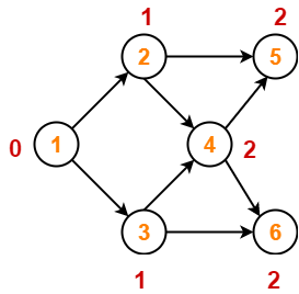
Step-01:


Write in-degree of each vertex-


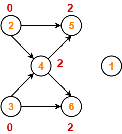
Step-02:


  • Vertex-1 has the least in-degree.
  • So, remove vertex-1 and its associated edges.
  • Now, update the in-degree of other vertices.


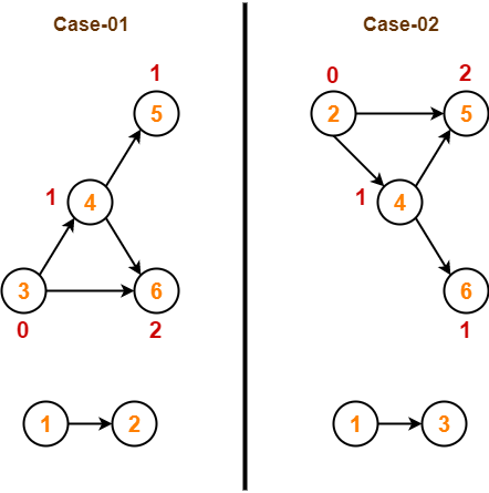
Step-03:


There are two vertices with the least in-degree. So, following 2 cases are possible-


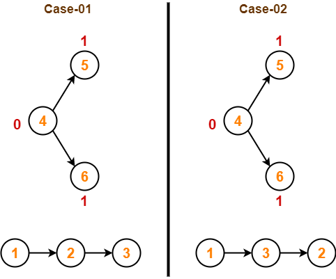
In case-01,

  • Remove vertex-2 and its associated edges.
  • Then, update the in-degree of other vertices.


In case-02,

  • Remove vertex-3 and its associated edges.
  • Then, update the in-degree of other vertices.


Step-04:


Now, the above two cases are continued separately in the similar manner.


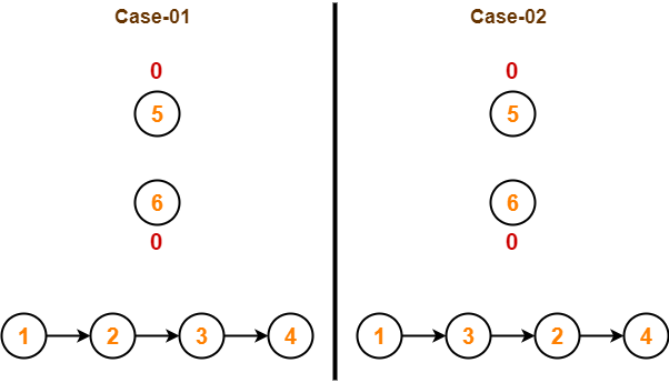
In case-01,

  • Remove vertex-3 since it has the least in-degree.
  • Then, update the in-degree of other vertices.


In case-02,

  • Remove vertex-2 since it has the least in-degree.
  • Then, update the in-degree of other vertices.


Step-05:


In case-01,

  • Remove vertex-4 since it has the least in-degree.
  • Then, update the in-degree of other vertices.


In case-02,

  • Remove vertex-4 since it has the least in-degree.
  • Then, update the in-degree of other vertices.


Step-06:


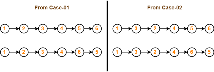
In case-01,

  • There are 2 vertices with the least in-degree.
  • So, 2 cases are possible.
  • Any of the two vertices may be taken first.


Same is with case-02.


Conclusion-


For the given graph, following 4 different topological orderings are possible-

  • 1 2 3 4 5 6
  • 1 2 3 4 6 5
  • 1 3 2 4 5 6
  • 1 3 2 4 6 5


Problem-03:


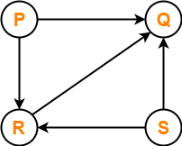
Consider the directed graph given below. Which of the following statements is true?


  1. The graph does not have any topological ordering.
  2. Both PQRS and SRPQ are topological orderings.
  3. Both PSRQ and SPRQ are topological orderings.
  4. PSRQ is the only topological ordering.


Solution-


  • The given graph is a directed acyclic graph.
  • So, topological orderings exist.
  • P and S must appear before R and Q in topological orderings as per the definition of topological sort.


Thus, Correct option is (C).


Problem-04:


Consider the following directed graph-


The number of different topological orderings of the vertices of the graph is ________ ?


Solution-


Number of different topological orderings possible = 6.

Thus, Correct answer is 6.


(The solution is explained in detail in the linked video lecture.)


To gain better understanding about Topological Sort,

Watch this Video Lecture


To practice previous years GATE problems on Topological Sort,

Watch this Video Lecture


Next Article- Shortest Path Problems


Other Popular Sorting Algorithms-


Get more notes and other study material of Design and Analysis of Algorithms.

Watch video lectures by visiting our YouTube channel LearnVidFun.