Month: July 2018

Construction of DFA | DFA Solved Examples

Construction Of DFA-


In this article, we will learn the construction of DFA.


Type-01 Problems-


In Type-01 problems, we will discuss the construction of DFA for languages consisting of strings ending with a particular substring.


Steps To Construct DFA-


Following steps are followed to construct a DFA for Type-01 problems-


Step-01:


  • Determine the minimum number of states required in the DFA.
  • Draw those states.


Use the following rule to determine the minimum number of states-


RULE

Calculate the length of substring.

All strings ending with ‘n’ length substring will always require minimum (n+1) states in the DFA.


Step-02:


  • Decide the strings for which DFA will be constructed.
  • The method for deciding the strings has been discussed in this Video.


Step-03:


  • Construct a DFA for the strings decided in Step-02.


Remember the following rule while constructing the DFA-


RULE

While constructing a DFA,

  • Always prefer to use the existing path.
  • Create a new path only when there exists no path to go with.


Step-04:


  • Send all the left possible combinations to the starting state.
  • Do not send the left possible combinations over the dead state.


PRACTICE PROBLEMS BASED ON CONSTRUCTION OF DFA-


Problem-01:


Draw a DFA for the language accepting strings ending with ’01’ over input alphabets ∑ = {0, 1}


Solution-


Regular expression for the given language = (0 + 1)*01


Step-01:


  • All strings of the language ends with substring “01”.
  • So, length of substring = 2.


Thus, Minimum number of states required in the DFA = 2 + 1 = 3.

It suggests that minimized DFA will have 3 states.


Step-02:


We will construct DFA for the following strings-

  • 01
  • 001
  • 0101


Step-03:


The required DFA is-


Problem-02:


Draw a DFA for the language accepting strings ending with ‘abb’ over input alphabets ∑ = {a, b}


Solution-


Regular expression for the given language = (a + b)*abb


Step-01:


  • All strings of the language ends with substring “abb”.
  • So, length of substring = 3.


Thus, Minimum number of states required in the DFA = 3 + 1 = 4.

It suggests that minimized DFA will have 4 states.


Step-02:


We will construct DFA for the following strings-

  • abb
  • aabb
  • ababb
  • abbabb


Step-03:


The required DFA is-


Problem-03:


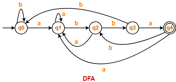
Draw a DFA for the language accepting strings ending with ‘abba’ over input alphabets ∑ = {a, b}


Solution-


Regular expression for the given language = (a + b)*abba


Step-01:


  • All strings of the language ends with substring “abba”.
  • So, length of substring = 4.


Thus, Minimum number of states required in the DFA = 4 + 1 = 5.

It suggests that minimized DFA will have 5 states.


Step-02:


We will construct DFA for the following strings-

  • abba
  • aabba
  • ababba
  • abbabba
  • abbaabba


Step-03:


The required DFA is-


Problem-04:


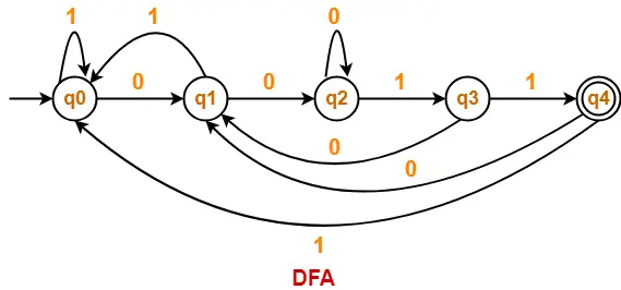
Draw a DFA for the language accepting strings ending with ‘0011’ over input alphabets ∑ = {0, 1}


Solution-


Regular expression for the given language = (0 + 1)*0011


Step-01:


  • All strings of the language ends with substring “0011”.
  • So, length of substring = 4.


Thus, Minimum number of states required in the DFA = 4 + 1 = 5.

It suggests that minimized DFA will have 5 states.


Step-02:


We will construct DFA for the following strings-

  • 0011
  • 00011
  • 000011
  • 0010011
  • 00110011


Step-03:


The required DFA is-


Also Read- Converting DFA to Regular Expression


To gain better understanding about Construction of DFA,

Watch this Video Lecture


Download Handwritten Notes Here-


Next Article- Construction of DFA | Type-02 Problems


Get more notes and other study material of Theory of Automata and Computation.

Watch video lectures by visiting our YouTube channel LearnVidFun.

Functional Dependency in DBMS

Functional Dependency-


In any relation, a functional dependency α → β holds if-

Two tuples having same value of attribute α also have same value for attribute β.


Mathematically,

If α and β are the two sets of attributes in a relational table R where-

  • α ⊆ R
  • β ⊆ R

Then, for a functional dependency to exist from α to β,

If t1[α] = t2[α], then t1[β] = t2[β]


α β
t1[α] t1[β]
t2[α] t2[β]
……. …….


fd : α → β


Types Of Functional Dependencies-


There are two types of functional dependencies-


  1. Trivial Functional Dependencies
  2. Non-trivial Functional Dependencies


1. Trivial Functional Dependencies-


  • A functional dependency X → Y is said to be trivial if and only if Y ⊆ X.
  • Thus, if RHS of a functional dependency is a subset of LHS, then it is called as a trivial functional dependency.


Examples-


The examples of trivial functional dependencies are-

  • AB → A
  • AB → B
  • AB → AB


2. Non-Trivial Functional Dependencies-


  • A functional dependency X → Y is said to be non-trivial if and only if Y ⊄ X.
  • Thus, if there exists at least one attribute in the RHS of a functional dependency that is not a part of LHS, then it is called as a non-trivial functional dependency.


Examples-


The examples of non-trivial functional dependencies are-

  • AB → BC
  • AB → CD


Inference Rules-


Reflexivity-

If B is a subset of A, then A → B always holds.


Transitivity-

If A → B and B → C, then A → C always holds.


Augmentation-

If A → B, then AC → BC always holds.


Decomposition-

If A → BC, then A → B and A → C always holds.


Composition-

If A → B and C → D, then AC → BD always holds.


Additive-

If A → B and A → C, then A → BC always holds.


Rules for Functional Dependency-


Rule-01:


A functional dependency X → Y will always hold if all the values of X are unique (different) irrespective of the values of Y.


Example-


Consider the following table-


A B C D E
5 4 3 2 2
8 5 3 2 1
1 9 3 3 5
4 7 3 3 8


The following functional dependencies will always hold since all the values of attribute ‘A’ are unique-

  • A → B
  • A → BC
  • A → CD
  • A → BCD
  • A → DE
  • A → BCDE

In general, we can say following functional dependency will always hold-


A → Any combination of attributes A, B, C, D, E


Similar will be the case for attributes B and E.


Rule-02:


A functional dependency X → Y will always hold if all the values of Y are same irrespective of the values of X.


Example-

Consider the following table-


A B C D E
5 4 3 2 2
8 5 3 2 1
1 9 3 3 5
4 7 3 3 8


The following functional dependencies will always hold since all the values of attribute ‘C’ are same-

  • A → C
  • AB → C
  • ABDE → C
  • DE → C
  • AE → C


In general, we can say following functional dependency will always hold true-


Any combination of attributes A, B, C, D, E → 


Combining Rule-01 and Rule-02 we can say-


In general, a functional dependency α → β always holds-

If either all values of α are unique or if all values of β are same or both.


Rule-03:


For a functional dependency X → Y to hold, if two tuples in the table agree on the value of attribute X, then they must also agree on the value of attribute Y.


Rule-04:


For a functional dependency X → Y, violation will occur only when for two or more same values of X, the corresponding Y values are different.


Next Article- Equivalence of Functional Dependencies


Get more notes and other study material of Database Management System (DBMS).

Watch video lectures by visiting our YouTube channel LearnVidFun.

Floyd Warshall Algorithm | Example | Time Complexity

Floyd Warshall Algorithm-


  • Floyd Warshall Algorithm is a famous algorithm.
  • It is used to solve All Pairs Shortest Path Problem.
  • It computes the shortest path between every pair of vertices of the given graph.
  • Floyd Warshall Algorithm is an example of dynamic programming approach.


Also Read- Shortest Path Problem


Advantages-


Floyd Warshall Algorithm has the following main advantages-

  • It is extremely simple.
  • It is easy to implement.


Algorithm-


Floyd Warshall Algorithm is as shown below-


Create a |V| x |V| matrix               // It represents the distance between every pair of vertices as given

For each cell (i,j) in M do-

    if i = = j

        M[ i ][ j ] = 0                 // For all diagonal elements, value = 0

    if (i , j) is an edge in E

        M[ i ][ j ] = weight(i,j)       // If there exists a direct edge between the vertices, value = weight of edge

    else

        M[ i ][ j ] = infinity          // If there is no direct edge between the vertices, value = ∞

for k from 1 to |V|

    for i from 1 to |V|

        for j from 1 to |V|

            if M[ i ][ j ] > M[ i ][ k ] + M[ k ][ j ]
            M[ i ][ j ] = M[ i ][ k ] + M[ k ][ j ]


Time Complexity-


  • Floyd Warshall Algorithm consists of three loops over all the nodes.
  • The inner most loop consists of only constant complexity operations.
  • Hence, the asymptotic complexity of Floyd Warshall algorithm is O(n3).
  • Here, n is the number of nodes in the given graph.


When Floyd Warshall Algorithm Is Used?


  • Floyd Warshall Algorithm is best suited for dense graphs.
  • This is because its complexity depends only on the number of vertices in the given graph.
  • For sparse graphs, Johnson’s Algorithm is more suitable.


PRACTICE PROBLEM BASED ON FLOYD WARSHALL ALGORITHM-


Problem-


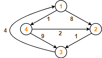
Consider the following directed weighted graph-


Using Floyd Warshall Algorithm, find the shortest path distance between every pair of vertices.


Solution-


Step-01:


  • Remove all the self loops and parallel edges (keeping the lowest weight edge) from the graph.
  • In the given graph, there are neither self edges nor parallel edges.


Step-02:


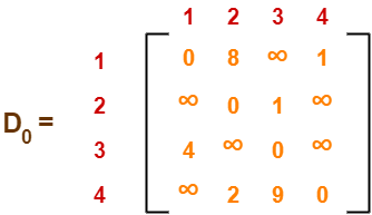
  • Write the initial distance matrix.
  • It represents the distance between every pair of vertices in the form of given weights.
  • For diagonal elements (representing self-loops), distance value = 0.
  • For vertices having a direct edge between them, distance value = weight of that edge.
  • For vertices having no direct edge between them, distance value = ∞.


Initial distance matrix for the given graph is-


Step-03:


Using Floyd Warshall Algorithm, write the following 4 matrices-


To learn how to write these matrices, watch this video here.

The last matrix D4 represents the shortest path distance between every pair of vertices.


Remember-


  • In the above problem, there are 4 vertices in the given graph.
  • So, there will be total 4 matrices of order 4 x 4 in the solution excluding the initial distance matrix.
  • Diagonal elements of each matrix will always be 0.


To gain better understanding about Floyd Warshall Algorithm,

Watch this Video Lecture


Next Article- Knapsack Problem


Get more notes and other study material of Design and Analysis of Algorithms.

Watch video lectures by visiting our YouTube channel LearnVidFun.
Quick Sort Algorithm | Example | Time Complexity

Quick Sort-


  • Quick Sort is a famous sorting algorithm.
  • It sorts the given data items in ascending order.
  • It uses the idea of divide and conquer approach.
  • It follows a recursive algorithm.


Quick Sort Algorithm-


Consider-

  • a = Linear Array in memory
  • beg = Lower bound of the sub array in question
  • end = Upper bound of the sub array in question


Then, Quick Sort Algorithm is as follows-


Partition_Array (a , beg , end , loc)


Begin

Set left = beg , right = end , loc = beg

Set done = false

While (not done) do

    While ( (a[loc] <= a[right] ) and (loc ≠ right) ) do

    Set right = right - 1

    end while


    if (loc = right) then

    Set done = true

    else if (a[loc] > a[right]) then

        Interchange a[loc] and a[right]

        Set loc = right

    end if


    if (not done) then

    While ( (a[loc] >= a[left] ) and (loc ≠ left) ) do

    Set left = left + 1

    end while


    if (loc = left) then

    Set done = true

    else if (a[loc] < a[left]) then

        Interchange a[loc] and a[left]

        Set loc = left

    end if

    end if

end while

End


How Does Quick Sort Works?


  • Quick Sort follows a recursive algorithm.
  • It divides the given array into two sections using a partitioning element called as pivot.


The division performed is such that-

  • All the elements to the left side of pivot are smaller than pivot.
  • All the elements to the right side of pivot are greater than pivot.


After dividing the array into two sections, the pivot is set at its correct position.

Then, sub arrays are sorted separately by applying quick sort algorithm recursively.


Quick Sort Example-


Consider the following array has to be sorted in ascending order using quick sort algorithm-


Quick Sort Algorithm works in the following steps-


Step-01:


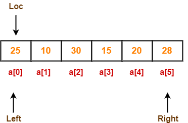
Initially-

  • Left and Loc (pivot) points to the first element of the array.
  • Right points to the last element of the array.


So to begin with, we set loc = 0, left = 0 and right = 5 as-


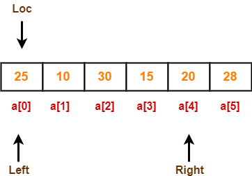
Step-02:


Since loc points at left, so algorithm starts from right and move towards left.

As a[loc] < a[right], so algorithm moves right one position towards left as-


Now, loc = 0, left = 0 and right = 4.


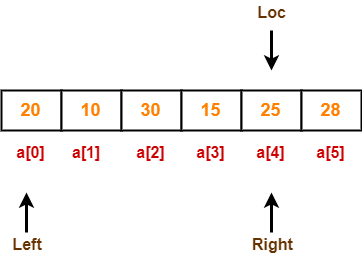
Step-03:


Since loc points at left, so algorithm starts from right and move towards left.

As a[loc] > a[right], so algorithm swaps a[loc] and a[right] and loc points at right as-


Now, loc = 4, left = 0 and right = 4.


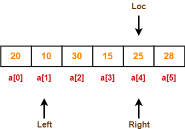
Step-04:


Since loc points at right, so algorithm starts from left and move towards right.

As a[loc] > a[left], so algorithm moves left one position towards right as-


Now, loc = 4, left = 1 and right = 4.


Step-05:


Since loc points at right, so algorithm starts from left and move towards right.

As a[loc] > a[left], so algorithm moves left one position towards right as-


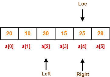
Now, loc = 4, left = 2 and right = 4.


Step-06:


Since loc points at right, so algorithm starts from left and move towards right.

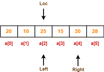
As a[loc] < a[left], so we algorithm swaps a[loc] and a[left] and loc points at left as-


Now, loc = 2, left = 2 and right = 4.


Step-07:


Since loc points at left, so algorithm starts from right and move towards left.

As a[loc] < a[right], so algorithm moves right one position towards left as-


Now, loc = 2, left = 2 and right = 3.


Step-08:


Since loc points at left, so algorithm starts from right and move towards left.

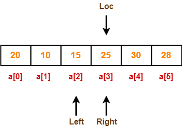
As a[loc] > a[right], so algorithm swaps a[loc] and a[right] and loc points at right as-


Now, loc = 3, left = 2 and right = 3.


Step-09:


Since loc points at right, so algorithm starts from left and move towards right.

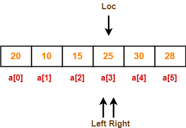
As a[loc] > a[left], so algorithm moves left one position towards right as-


Now, loc = 3, left = 3 and right = 3.


Now,

  • loc, left and right points at the same element.
  • This indicates the termination of procedure.
  • The pivot element 25 is placed in its final position.
  • All elements to the right side of element 25 are greater than it.
  • All elements to the left side of element 25 are smaller than it.


Now, quick sort algorithm is applied on the left and right sub arrays separately in the similar manner.


Quick Sort Analysis-


  • To find the location of an element that splits the array into two parts, O(n) operations are required.
  • This is because every element in the array is compared to the partitioning element.
  • After the division, each section is examined separately.
  • If the array is split approximately in half (which is not usually), then there will be log2n splits.
  • Therefore, total comparisons required are f(n) = n x log2n = O(nlog2n).


Order of Quick Sort = O(nlog2n)


Worst Case-


  • Quick Sort is sensitive to the order of input data.
  • It gives the worst performance when elements are already in the ascending order.
  • It then divides the array into sections of 1 and (n-1) elements in each call.
  • Then, there are (n-1) divisions in all.
  • Therefore, here total comparisons required are f(n) = n x (n-1) = O(n2).


Order of Quick Sort in worst case = O(n2)


Advantages of Quick Sort-


The advantages of quick sort algorithm are-

  • Quick Sort is an in-place sort, so it requires no temporary memory.
  • Quick Sort is typically faster than other algorithms.

(because its inner loop can be efficiently implemented on most architectures)

  • Quick Sort tends to make excellent usage of the memory hierarchy like virtual memory or caches.
  • Quick Sort can be easily parallelized due to its divide and conquer nature.


Disadvantages of Quick Sort-


The disadvantages of quick sort algorithm are-

  • The worst case complexity of quick sort is O(n2).
  • This complexity is worse than O(nlogn) worst case complexity of algorithms like merge sort, heap sort etc.
  • It is not a stable sort i.e. the order of equal elements may not be preserved.


To gain better understanding about Quick Sort Algorithm,

Watch this Video Lecture


Next Article- Topological Sort


Other Popular Sorting Algorithms-


Get more notes and other study material of Design and Analysis of Algorithms.

Watch video lectures by visiting our YouTube channel LearnVidFun.
Binary Search Algorithm | Example | Time Complexity

Searching-


  • Searching is a process of finding a particular element among several given elements.
  • The search is successful if the required element is found.
  • Otherwise, the search is unsuccessful.


Searching Algorithms-


Searching Algorithms are a family of algorithms used for the purpose of searching.

The searching of an element in the given array may be carried out in the following two ways-


  1. Linear Search
  2. Binary Search


In this article, we will discuss about Binary Search Algorithm.


Binary Search-


  • Binary Search is one of the fastest searching algorithms.
  • It is used for finding the location of an element in a linear array.
  • It works on the principle of divide and conquer technique.


Binary Search Algorithm can be applied only on Sorted arrays.


So, the elements must be arranged in-

  • Either ascending order if the elements are numbers.
  • Or dictionary order if the elements are strings.


To apply binary search on an unsorted array,

  • First, sort the array using some sorting technique.
  • Then, use binary search algorithm.


Also Read- Linear Search


Binary Search Algorithm-


Consider-

  • There is a linear array ‘a’ of size ‘n’.
  • Binary search algorithm is being used to search an element ‘item’ in this linear array.
  • If search ends in success, it sets loc to the index of the element otherwise it sets loc to -1.
  • Variables beg and end keeps track of the index of the first and last element of the array or sub array in which the element is being searched at that instant.
  • Variable mid keeps track of the index of the middle element of that array or sub array in which the element is being searched at that instant.


Then, Binary Search Algorithm is as follows-


Begin

Set beg = 0

Set end = n-1

Set mid = (beg + end) / 2

while ( (beg <= end) and (a[mid] ≠ item) ) do

    if (item < a[mid]) then

        Set end = mid - 1

    else

        Set beg = mid + 1

    endif

Set mid = (beg + end) / 2

endwhile

if (beg > end) then

    Set loc = -1

else

    Set loc = mid

endif

End


Explanation


Binary Search Algorithm searches an element by comparing it with the middle most element of the array.

Then, following three cases are possible-


Case-01


If the element being searched is found to be the middle most element, its index is returned.


Case-02


If the element being searched is found to be greater than the middle most element,

then its search is further continued in the right sub array of the middle most element.


Case-03


If the element being searched is found to be smaller than the middle most element,

then its search is further continued in the left sub array of the middle most element.


This iteration keeps on repeating on the sub arrays until the desired element is found

or size of the sub array reduces to zero.


Time Complexity Analysis-


Binary Search time complexity analysis is done below-

  • In each iteration or in each recursive call, the search gets reduced to half of the array.
  • So for n elements in the array, there are log2n iterations or recursive calls.


Thus, we have-


Time Complexity of Binary Search Algorithm is O(log2n).

Here, n is the number of elements in the sorted linear array.


This time complexity of binary search remains unchanged irrespective of the element position even if it is not present in the array.


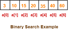
Binary Search Example-


Consider-

  • We are given the following sorted linear array.
  • Element 15 has to be searched in it using Binary Search Algorithm.


Binary Search Algorithm works in the following steps-


Step-01:


  • To begin with, we take beg=0 and end=6.
  • We compute location of the middle element as-

mid

= (beg + end) / 2

= (0 + 6) / 2

= 3

  • Here, a[mid] = a[3] = 20 ≠ 15 and beg < end.
  • So, we start next iteration.


Step-02:


  • Since a[mid] = 20 > 15, so we take end = mid – 1 = 3 – 1 = 2 whereas beg remains unchanged.
  • We compute location of the middle element as-

mid

= (beg + end) / 2

= (0 + 2) / 2

= 1

  • Here, a[mid] = a[1] = 10 ≠ 15 and beg < end.
  • So, we start next iteration.


Step-03:


  • Since a[mid] = 10 < 15, so we take beg = mid + 1 = 1 + 1 = 2 whereas end remains unchanged.
  • We compute location of the middle element as-

mid

= (beg + end) / 2

= (2 + 2) / 2

= 2

  • Here, a[mid] = a[2] = 15 which matches to the element being searched.
  • So, our search terminates in success and index 2 is returned.


Binary Search Algorithm Advantages-


The advantages of binary search algorithm are-

  • It eliminates half of the list from further searching by using the result of each comparison.
  • It indicates whether the element being searched is before or after the current position in the list.
  • This information is used to narrow the search.
  • For large lists of data, it works significantly better than linear search.


Binary Search Algorithm Disadvantages-


The disadvantages of binary search algorithm are-

  • It employs recursive approach which requires more stack space.
  • Programming binary search algorithm is error prone and difficult.
  • The interaction of binary search with memory hierarchy i.e. caching is poor.

(because of its random access nature)


Important Note-


For in-memory searching, if the interval to be searched is small,

  • Linear search may exhibit better performance than binary search.
  • This is because it exhibits better locality of reference.


To gain better understanding about Binary Search Algorithm,

Watch this Video Lecture


Next Article- Selection Sort


Get more notes and other study material of Design and Analysis of Algorithms.

Watch video lectures by visiting our YouTube channel LearnVidFun.